


1. Select all
As someone who sorts data quite often, I find using the select all button really helps to ensure you are sorting on all columns and rows. There is nothing worse than spending hours working on a large dataset only to realise somewhere along the way you sorted on just some of the columns and all your data has become misaligned. To select all the cells in a table simply click the triangle in the corner of your spreadsheet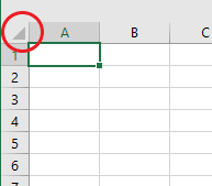
2. Freezing columns and rows
When dealing with large spreadsheets full of data it is sometimes hard to remember what information is in each column, but by freezing the top row, you are able to scroll down your spreadsheet while the top row remains stationary. To do this click on the view tab at the top of excel then Freeze panes, you can then determine whether to freeze the top row, first column or multiple columns depending on your current selection.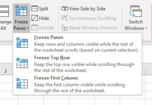
3. Autofill and Flash fill
These are both great time savers, as they make filling in cells with the same data or a pattern much easier. For example, if you type the date in one cell and then want to carry that on down through the column, you start by typing the date then move the cursor to the bottom-right corner of the cell. When a plus sign appears (+), click and drag down to select all the cells you need to fill. You can also highlight the cells you want to fill by clicking the fill button of the Home tab, this will give you various options including a flash fill.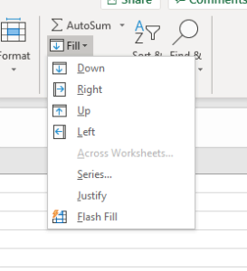 Flash fill is where Excel will look for patterns in the data as you enter it and try to continue the pattern and fill in subsequent cells for you. Excel will sometimes suggest a flash fill to you if the pattern is obvious and you just need to click enter for the flash fill to happen. If Excel doesn’t suggest a fill you can go to the Fill button on the Home tab and choose Flash Fill.
4. Pivot Tables
Pivot tables are a great way of summarising data from complex and lengthy spreadsheets. To create one it is important that all columns and rows are properly titled then click PivotTable on the insert tab, which will create a new sheet on your spreadsheet containing the PivotTable wizard, where you can build your table. If you are unsure where to begin Excel can recommend a PivotTable for you. Both options can be found on the insert tab.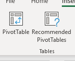
5. Wrap text/merge and center
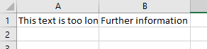
I have grouped these two tips as I think they both fall into a similar category. Let’s start with Wrap Text, this can be used where the contents of the cell is longer than the width of the cell. By wrapping the text you can display longer text in a cell without it overflowing to other cells. It displays the cell contents on multiple lines, rather than one long line. To wrap text simply chose the cell you want to wrap and on the Home tab chose the Wrap Text button. Below is an example of the wrapped and not wrapped text.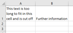
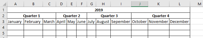
 Merging and centering can be used for when a title is to be centred over a particular section of a spreadsheet, or if you want multiple rows to be grouped together. It is important to note that when a group of cells is merged, only the text in the upper-leftmost box is preserved. To Merge and Centre choose the cells you want to merge then on the Home tab click the Merge and Center button.
6. Text to columns
I use this functionality all the time, it is very useful when you have multiple rows of data in one column that needs to be split across multiple columns. See below for an example of before using text to a column and after.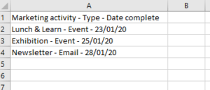
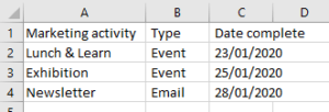 To use Text to Columns, highlight the column you want to split (making sure the fields after it are empty so they don’t get overwritten) and click the Text to Columns button on the Data tab.
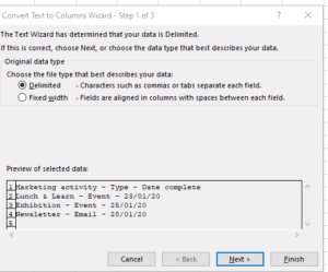
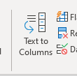 This will bring up a wizard that will help you to split the columns either by fixed width or by using a delimiter. The wizard contains more instructions on how to pick the right option for you.
7. Concatenate data
Concatenation is really the reverse of the Text to Columns functionality it is pulling data from multiple columns into one column (and I use it just as often as Text to Columns!) To concatenate data you need to choose an empty field that you would like your data to be in and then click on the function button. You can then search for the function by typing Concatenate.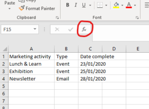 This will then bring up a wizard that allows you to choose which columns you want to bring together, you can add multiple columns. It’s worth noting you might need to create a column with a space in it so the data isn’t put together with no spaces (ExhibitionEvent23/01/20 instead of Exhibition Event 23/01/20).
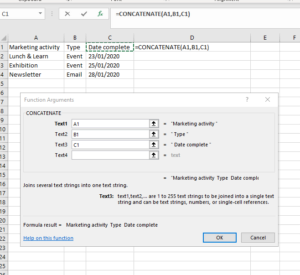 See left for an image of function wizard. Another point to consider is that the field you have created will be a formula field so if you want to remove the fields you have concatenated to just leave one field with all the information it is important to copy the field and then click paste value. This will stop the field being a formula field and you will be able to delete the redundant columns.
8. Removing duplicates
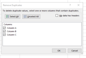
This is a useful tool when working on a large data file where you want to remove duplicate values from a column. To do this highlight your data click on the Data tab and click on Remove Duplicates. This then brings up a wizard where you can identify which column you want to remove duplicates from, once you click ok excel will remove any duplicate rows from your data.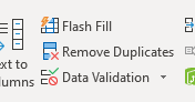
9. Highlight duplicates
This is a useful tool when you don’t want to remove duplicates from your data but you do want to highlight them. To do this you will need to highlight the column(s) you want to check for duplicates and then click on Conditional Formatting. You then hover your mouse over Highlight Cell Rules and go down to Duplicate Values. This will then change all fields with a duplicate to a red field. There are many other useful options in the highlight cell rules section you might want to explore. I usually then sort my spreadsheet and instead of sorting on the value I sort on cell colour to bring all my duplicated highlighted cells to the top so I can work on them accordingly.
10. Charts/graphs
 The chart and graph functionality in excel is very useful for presenting data in a more digestible format. When you are first starting out using charts I would advise using the Recommended Charts functionality where excel guesses based on your dataset which chart is most appropriate. To use this highlight the columns you want to be included in your chart click on the Insert tab then click on Recommended Charts. You can then decide whether to use Excels recommended chart or choose your own from all charts. Once you click ok you can add further detail to your chart like titles or adapt what data goes on which axis.
Some of these tips you may already know but you may hopefully there are a couple of tricks that are new to you this year.
Take a look at our blog for other IT tips
The chart and graph functionality in excel is very useful for presenting data in a more digestible format. When you are first starting out using charts I would advise using the Recommended Charts functionality where excel guesses based on your dataset which chart is most appropriate. To use this highlight the columns you want to be included in your chart click on the Insert tab then click on Recommended Charts. You can then decide whether to use Excels recommended chart or choose your own from all charts. Once you click ok you can add further detail to your chart like titles or adapt what data goes on which axis.
Some of these tips you may already know but you may hopefully there are a couple of tricks that are new to you this year.
Take a look at our blog for other IT tips